Pandas Fundamentals - I

This notebook was created by Ryan Abernathey (© Copyright 2016-2021) and is part of the An Introduction to Earth and Environmental Data Science textbook.

All content in this book (ie, any files and content in the content/ folder) is licensed under the Creative Commons Attribution-ShareAlike 4.0 International (CC BY-SA 4.0) license.

This notebook demonstrates basic features of the pandas python package.

Pandas is an extension to python, so we first have to import the package before we can run anything else.

import pandas as pd
import numpy as np
from matplotlib import pyplot as plt
%matplotlib inline

Pandas Data Structures: Series

A Series represents a one-dimensional array of data. The main difference between a Series and numpy array is that a Series has an index. The index contains the labels that we use to access the data.

There are many ways to create a Series. We will just show a few.

(Data are from the NASA Planetary Fact Sheet.)

names = ['Mercury', 'Venus', 'Earth']
values = [0.3e24, 4.87e24, 5.97e24]
masses = pd.Series(values, index=names)
masses

Mercury    3.000000e+23
Venus      4.870000e+24
Earth      5.970000e+24
dtype: float64

Series have built in plotting methods.

masses.plot(kind='bar')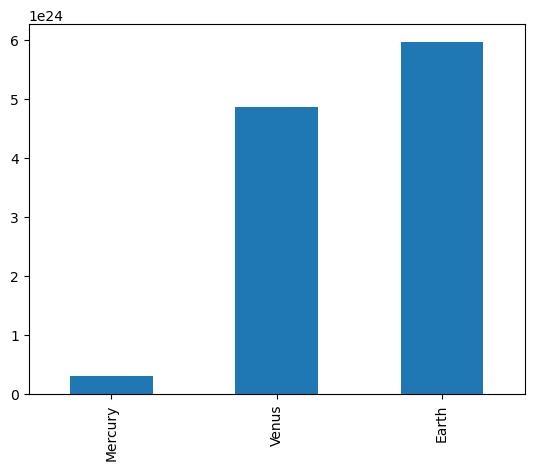

Arithmetic operations and most numpy function can be applied to Series. An important point is that the Series keep their index during such operations.

np.log(masses) / masses**2

Mercury    6.006452e-46
Venus      2.396820e-48
Earth      1.600655e-48
dtype: float64

We can access the underlying index object if we need to:

masses.index

Index(['Mercury', 'Venus', 'Earth'], dtype='str')

Indexing

We can get values back out using the index via the .loc attribute

masses.loc['Earth']

np.float64(5.97e+24)

Or by raw position using .iloc

masses.iloc[2]

np.float64(5.97e+24)

We can pass a list or array to loc to get multiple rows back:

masses.loc[['Venus', 'Earth']]

Venus    4.870000e+24
Earth    5.970000e+24
dtype: float64

And we can even use slice notation

masses.loc['Mercury':'Earth']

Mercury    3.000000e+23
Venus      4.870000e+24
Earth      5.970000e+24
dtype: float64

masses.iloc[:2]

Mercury    3.000000e+23
Venus      4.870000e+24
dtype: float64

If we need to, we can always get the raw data back out as well

masses.values # a numpy array

array([3.00e+23, 4.87e+24, 5.97e+24])

masses.index # a pandas Index object

Index(['Mercury', 'Venus', 'Earth'], dtype='str')

Pandas Data Structures: DataFrame

There is a lot more to Series, but they are limit to a single “column”. A more useful Pandas data structure is the DataFrame. A DataFrame is basically a bunch of series that share the same index. It’s a lot like a table in a spreadsheet.

Below we create a DataFrame.

# first we create a dictionary
data = {'mass': [0.3e24, 4.87e24, 5.97e24],       # kg
        'diameter': [4879e3, 12_104e3, 12_756e3], # m
        'rotation_period': [1407.6, np.nan, 23.9] # h
       }
df = pd.DataFrame(data, index=['Mercury', 'Venus', 'Earth'])
df

	mass	diameter	rotation_period
Mercury	3.000000e+23	4879000.0	1407.6
Venus	4.870000e+24	12104000.0	NaN
Earth	5.970000e+24	12756000.0	23.9

Pandas handles missing data very elegantly, keeping track of it through all calculations.

df.info()

<class 'pandas.DataFrame'>
Index: 3 entries, Mercury to Earth
Data columns (total 3 columns):
 #   Column           Non-Null Count  Dtype  
---  ------           --------------  -----  
 0   mass             3 non-null      float64
 1   diameter         3 non-null      float64
 2   rotation_period  2 non-null      float64
dtypes: float64(3)
memory usage: 113.0 bytes

A wide range of statistical functions are available on both Series and DataFrames.

df.min()

mass               3.000000e+23
diameter           4.879000e+06
rotation_period    2.390000e+01
dtype: float64

df.mean()

mass               3.713333e+24
diameter           9.913000e+06
rotation_period    7.157500e+02
dtype: float64

df.std()

mass               3.006765e+24
diameter           4.371744e+06
rotation_period    9.784237e+02
dtype: float64

df.describe()

	mass	diameter	rotation_period
count	3.000000e+00	3.000000e+00	2.000000
mean	3.713333e+24	9.913000e+06	715.750000
std	3.006765e+24	4.371744e+06	978.423653
min	3.000000e+23	4.879000e+06	23.900000
25%	2.585000e+24	8.491500e+06	369.825000
50%	4.870000e+24	1.210400e+07	715.750000
75%	5.420000e+24	1.243000e+07	1061.675000
max	5.970000e+24	1.275600e+07	1407.600000

We can get a single column as a Series using python’s getitem syntax on the DataFrame object.

df['mass']

Mercury    3.000000e+23
Venus      4.870000e+24
Earth      5.970000e+24
Name: mass, dtype: float64

…or using attribute syntax.

df.mass

Mercury    3.000000e+23
Venus      4.870000e+24
Earth      5.970000e+24
Name: mass, dtype: float64

Indexing works very similar to series

df.loc['Earth']

mass               5.970000e+24
diameter           1.275600e+07
rotation_period    2.390000e+01
Name: Earth, dtype: float64

df.iloc[2]

mass               5.970000e+24
diameter           1.275600e+07
rotation_period    2.390000e+01
Name: Earth, dtype: float64

But we can also specify the column we want to access

df.loc['Earth', 'mass']

np.float64(5.97e+24)

df.iloc[:2, 0]

Mercury    3.000000e+23
Venus      4.870000e+24
Name: mass, dtype: float64

If we make a calculation using columns from the DataFrame, it will keep the same index:

volume =  4/3 * np.pi * (df.diameter/2)**3
df.mass / volume

Mercury    4933.216530
Venus      5244.977070
Earth      5493.285577
dtype: float64

Which we can easily add as another column to the DataFrame:

df['density'] = df.mass / volume
df

	mass	diameter	rotation_period	density
Mercury	3.000000e+23	4879000.0	1407.6	4933.216530
Venus	4.870000e+24	12104000.0	NaN	5244.977070
Earth	5.970000e+24	12756000.0	23.9	5493.285577

Merging Data

Pandas supports a wide range of methods for merging different datasets. These are described extensively in the documentation. Here we just give a few examples.

temperature = pd.Series([167, 464, 15, -65],
                     index=['Mercury', 'Venus', 'Earth', 'Mars'],
                     name='temperature')
temperature

Mercury    167
Venus      464
Earth       15
Mars       -65
Name: temperature, dtype: int64

# returns a new DataFrame
df.join(temperature)

	mass	diameter	rotation_period	density	temperature
Mercury	3.000000e+23	4879000.0	1407.6	4933.216530	167
Venus	4.870000e+24	12104000.0	NaN	5244.977070	464
Earth	5.970000e+24	12756000.0	23.9	5493.285577	15

# returns a new DataFrame
df.join(temperature, how='right')

	mass	diameter	rotation_period	density	temperature
Mercury	3.000000e+23	4879000.0	1407.6	4933.216530	167
Venus	4.870000e+24	12104000.0	NaN	5244.977070	464
Earth	5.970000e+24	12756000.0	23.9	5493.285577	15
Mars	NaN	NaN	NaN	NaN	-65

# returns a new DataFrame
everyone = df.reindex(['Mercury', 'Venus', 'Earth', 'Mars'])
everyone

	mass	diameter	rotation_period	density
Mercury	3.000000e+23	4879000.0	1407.6	4933.216530
Venus	4.870000e+24	12104000.0	NaN	5244.977070
Earth	5.970000e+24	12756000.0	23.9	5493.285577
Mars	NaN	NaN	NaN	NaN

We can also index using a boolean series. This is very useful

adults = df[df.mass > 4e24]
adults

	mass	diameter	rotation_period	density
Venus	4.870000e+24	12104000.0	NaN	5244.977070
Earth	5.970000e+24	12756000.0	23.9	5493.285577

df['is_big'] = df.mass > 4e24
df

	mass	diameter	rotation_period	density	is_big
Mercury	3.000000e+23	4879000.0	1407.6	4933.216530	False
Venus	4.870000e+24	12104000.0	NaN	5244.977070	True
Earth	5.970000e+24	12756000.0	23.9	5493.285577	True

Modifying Values

We often want to modify values in a dataframe based on some rule. To modify values, we need to use .loc or .iloc

df.loc['Earth', 'mass'] = 5.98+24
df.loc['Venus', 'diameter'] += 1
df

	mass	diameter	rotation_period	density	is_big
Mercury	3.000000e+23	4879000.0	1407.6	4933.216530	False
Venus	4.870000e+24	12104001.0	NaN	5244.977070	True
Earth	2.998000e+01	12756000.0	23.9	5493.285577	True

Plotting

DataFrames have all kinds of useful plotting built in.

df.plot(kind='scatter', x='mass', y='diameter', grid=True)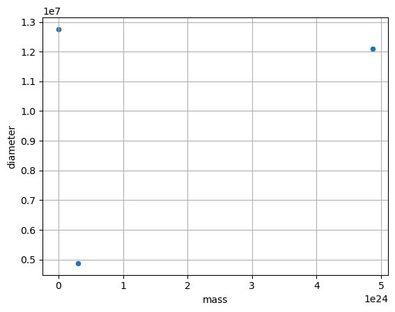

df.plot(kind='bar')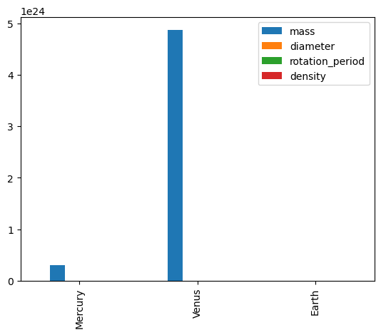

Reading Data Files: Palmer Penguin Data

In this example, we will use data from the Palmer Archipelago Penguins. This dataset has become a popular example dataset for environmental analysis, because it is comparatively simple to understand and has some nice features for analysis. (see e.g. here)

These data were collected from 2007 - 2009 by Dr. Kristen Gorman with the Palmer Station Long Term Ecological Research Program, part of the US Long Term Ecological Research Network. The data are originally from the Environmental Data Initiative (EDI) Data Portal, and are available for use by CC0 license (“No Rights Reserved”) in accordance with the Palmer Station Data Policy.

To read it into pandas, we will use the read_csv function. This function is incredibly complex and powerful. You can use it to extract data from almost any text file. However, you need to understand how to use its various options.

df_penguins = pd.read_csv('../Data/palmer_penguin_data.csv')
df_penguins

						Data originally published in:  Gorman KB	Williams TD	Fraser WR (2014). Ecological sexual dimorphism and environmental variability within a community of Antarctic penguins (genus Pygoscelis). PLoS ONE 9(3):e90081. https://doi.org/10.1371/journal.pone.0090081
rowid	species	island	bill_length_mm	bill_depth_mm	flipper_length_mm	body_mass_g	sex	year
1	Adelie	Torgersen	39.1	18.7	181	3750	male	2007
2	Adelie	Torgersen	39.5	17.4	186	3800	female	2007
3	Adelie	Torgersen	40.3	18	195	3250	female	2007
4	Adelie	Torgersen	nan	nan	nan	NaN	NaN	2007
...	...	...	...	...	...	...	...	...
340	Chinstrap	Dream	55.8	19.8	207	4000	male	2009
341	Chinstrap	Dream	43.5	18.1	202	3400	female	2009
342	Chinstrap	Dream	49.6	18.2	193	3775	male	2009
343	Chinstrap	Dream	50.8	19	210	4100	male	2009
344	Chinstrap	Dream	50.2	18.7	198	3775	female	2009

345 rows × 3 columns

This does not look right. It looks like that there is an extra line at the top, with some information about the dataset. We also see that there is some data that seems to be missing. If we look directly into the csv, we see that these are indicated with "NA" This is something that we should address directly.

The pd.read_csv() method has many options for ingesting data:

import pandas as pd
df_penguins = pd.read_csv('../Data/palmer_penguin_data.csv',
                          sep = ',',
                          na_values='NA',
                          skiprows= 1,
                          )
df_penguins

df_penguins.head()

	rowid	species	island	bill_length_mm	bill_depth_mm	flipper_length_mm	body_mass_g	sex	year
0	1	Adelie	Torgersen	39.1	18.7	181.0	3750.0	male	2007
1	2	Adelie	Torgersen	39.5	17.4	186.0	3800.0	female	2007
2	3	Adelie	Torgersen	40.3	18.0	195.0	3250.0	female	2007
3	4	Adelie	Torgersen	NaN	NaN	NaN	NaN	NaN	2007
4	5	Adelie	Torgersen	36.7	19.3	193.0	3450.0	female	2007

This looks better

Great. The missing data is now represented by NaN.

What data types did pandas infer?

df_penguins.info()

<class 'pandas.DataFrame'>
RangeIndex: 344 entries, 0 to 343
Data columns (total 9 columns):
 #   Column             Non-Null Count  Dtype  
---  ------             --------------  -----  
 0   rowid              344 non-null    int64  
 1   species            344 non-null    str    
 2   island             344 non-null    str    
 3   bill_length_mm     342 non-null    float64
 4   bill_depth_mm      342 non-null    float64
 5   flipper_length_mm  342 non-null    float64
 6   body_mass_g        342 non-null    float64
 7   sex                333 non-null    str    
 8   year               344 non-null    int64  
dtypes: float64(4), int64(2), str(3)
memory usage: 30.2 KB

Quick Statistics

We can calculate basic statistics for columns that are numeric. We can see that this simply skips any columns with text.

df_penguins.describe()

	rowid	bill_length_mm	bill_depth_mm	flipper_length_mm	body_mass_g	year
count	344.000000	342.000000	342.000000	342.000000	342.000000	344.000000
mean	172.500000	43.921930	17.151170	200.915205	4201.754386	2008.029070
std	99.448479	5.459584	1.974793	14.061714	801.954536	0.818356
min	1.000000	32.100000	13.100000	172.000000	2700.000000	2007.000000
25%	86.750000	39.225000	15.600000	190.000000	3550.000000	2007.000000
50%	172.500000	44.450000	17.300000	197.000000	4050.000000	2008.000000
75%	258.250000	48.500000	18.700000	213.000000	4750.000000	2009.000000
max	344.000000	59.600000	21.500000	231.000000	6300.000000	2009.000000

For columns with text, we can get counts on how often each value occurs. Calculating this for numeric columns does not make sense, so we only select the columns that contain text.

text_columns = ['species', 'island', 'sex']
df_penguins[text_columns].value_counts()

species    island     sex   
Gentoo     Biscoe     male      61
                      female    58
Chinstrap  Dream      female    34
                      male      34
Adelie     Dream      male      28
                      female    27
           Torgersen  female    24
                      male      23
           Biscoe     female    22
                      male      22
Name: count, dtype: int64

We can now see that there are thee penguin species in the dataset. The Adelie penguin is the only penguin that is found on all three islands (Biscoe, Dream, Torgersen). We also get counts of the sex for each species and island.