Time Series Analysis - Introduction
Motivation
Specific learning goals
Concepts:
Skills:
Recap: Tabular data
We have already learned about tabular data, which is a type of structured data. Tabular data is organized in rows and columns, where each column represents a feature and each row represents a value. For example, the Palmer Penguin dataset is a tabular dataset that contains measurements of penguin species, island, bill length, bill depth, flipper length, body mass, and sex.
In the case of the Palmer Penguin dataset, we have a population sample that is drawn from a larger population of penguins. We can use this dataset to explore the relationships between different features, such as how bill length varies across different species of penguins (Figure 1) and then make inferences about the entire population.

One important thing to note is that there is no particular order in the data. The rows can be arranged in any order without affecting the analysis. For example, we can sort the rows by bill length, but this does not change the underlying relationships between the features.
Time series data
Time series data is a specific type of tabular data where the rows represent measurements taken at different points in time. The columns can represent different features or variables that are measured at each time point. This means that unlike the Palmer Penguin dataset, there is a specific order to the rows in time series data, as they represent measurements taken at different time points.
Because there is order, we need to apply different techniques to analyze time series data compared to other types of tabular data.
Take for example the time series of atmospheric CO\(_2\) at the Mauna Loa Observatory in Hawaii (Figure 2):
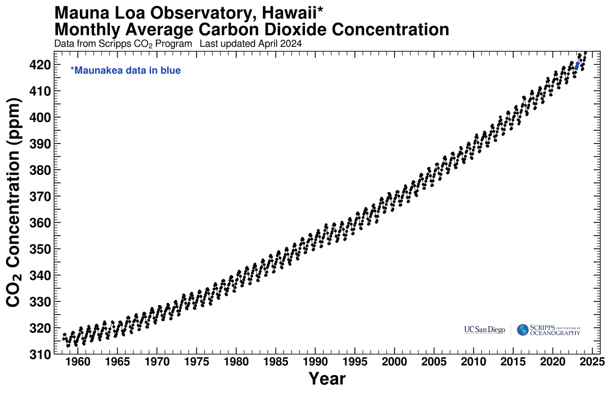
Here, the order clearly matters. If we were to shuffle the rows of this dataset, we would lose the temporal structure and the underlying trends and patterns in the data. For example, we would not be able to identify the long-term increase in CO\(_2\) levels or the seasonal fluctuations that are present in the data.
In addition to the trend within the data, we can also identify other patterns such as seasonality, which is a regular pattern that repeats over a specific period of time (e.g. annually).
Features of time series data
- Trend: A long-term increase or decrease in the data. For example, the long-term increase in CO\(_2\) levels in the Mauna Loa dataset.
- Periodicity: A regular pattern that repeats over a specific period of time. For example, the seasonal fluctuations in CO\(_2\) levels in the Mauna Loa dataset.
- Autocorrelation: The correlation of a time series with its own past values. For example, if we have a time series of daily temperatures, we might find that today’s temperature is correlated with yesterday’s temperature. Similarly, tomorrows temperature might be correlated with today’s temperature AND yesterdays temperature (but a bit less than the correlation with today’s temperature).
Therefore, if we were to build a model to predict future CO\(_2\) levels based on the Mauna Loa dataset, we would need to take into account these features of the data.
For example, we could use a model that captures the trend, such as a linear regression model, to predict the long-term increase in CO\(_2\) levels and then add a seasonal component to capture the periodic fluctuations:
We could use a additive model for the total CO\(_2\) levels, which would be the sum of the base level , the trend (the long-term increase), and the seasonality (the periodic fluctuations):
Total CO\(_2\) = Base Level + Trend + Seasonality
Dealing with data gaps
Because time series data is often collected at regular intervals, it is common to encounter gaps in the data due to missing observations. These gaps can arise from various reasons, such as sensor malfunctions, data transmission errors, or simply the absence of measurements.
To deal with data gaps in time series data, we can use several techniques:
Interpolation: This involves estimating the missing values based on the available data. Common interpolation methods include linear interpolation, spline interpolation, and polynomial interpolation.
Forward/Backward Filling: This technique involves filling missing values with the last available observation (forward filling) or the next available observation (backward filling). This is particularly useful for time series data where the last known value is a reasonable estimate for the missing value.
Imputation: More advanced statistical techniques can be used to estimate missing values based on the relationships between different variables in the dataset. This can include methods such as k-nearest neighbors (KNN) imputation or regression imputation.
Removing Missing Values: In some cases, it may be appropriate to simply remove rows with missing values from the dataset.
Time series data in pandas
Luckily, the pandas library in Python has built-in functionalities to handle time series data, which we will now explore using weather station data from the NOAA Global Historical Climatology Network (GHCN).