flowchart LR
  A(Environmental Issue) --> B(Specific Question)
  B --> C(Data Analysis Workflow)
  B1[Environmental Data] --> C
  C --> D(Product)
Gridded data and weather effects
Background
Learning Goals
Aside: Reproducible workflows and data integration
You have already seen a schematic representation of the data analysis process(Figure 1).
So far, we have been mainly working with data that was manually downloaded, distributed as a files through our shared repository, and then loaded into pandas or xarray for analysis.
From a reproducibility perspective, this is not ideal. We have to manually download data, which is not reproducible and also not scalable. We also don’t control what happens to the data after we download it, which can lead to issues with data integrity and version control.
There are several tools and packages that can help us to make this process more reproducible and scalable.
Automating data download and access
The pooch library, allows us to automate the process of downloading data from a remote location and caching it locally. It also calculates/ checks a unique hash for each file, which allows us to verify the integrity of the data and to ensure that we are using the correct version of the data.
import pooch
import xarray as xr

POOCH = pooch.create(
    path=pooch.os_cache("greenland_ice_sheet"),
    base_url="https://zenodo.org/record/4977910/files/",
    registry={
        "vel_2010-07-01_2011-06-31.nc": "md5:80ad1a3c381af185069bc032a6459745",
    }
)

fname = POOCH.fetch("vel_2010-07-01_2011-06-31.nc")
fname

ds = xr.open_dataset(fname)
Downloading file 'vel_2010-07-01_2011-06-31.nc' from 'https://zenodo.org/record/4977910/files/vel_2010-07-01_2011-06-31.nc' to '/home/runner/.cache/greenland_ice_sheet'.Loading data over a network
- Pandas and xarray also allow us to load data directly from a remote location without having to download it first.
- This also allows us to work with datasets that are located on servers such as Amazon Web Services (AWS) or Google Cloud Storage (GCS) without having to download the data to our local machine.
Environmental data on AWS (and other cloud providers)
Many environmental datasets are now available on cloud platforms such as Amazon Web Services (AWS), Microsoft Azure, or Google Cloud Storage (GCS).
For example, all NOAA Climate Data Records (CDR) data are available freely to the public via NOAA National Centers for Environmental Information. Recently, the NOAA Open Data Dissemination Program also made all NOAA CDRs available on three major commercial cloud service providers (i.e., Amazon Web Service, Google Cloud, and Microsoft Azure). The NOAA Climate Data Records (CDRs) are available to anyone interested in accessing the data and are typically free of charge.
Satellite data

There are many environmental datasets available.
This link contains a table with many datasets: Climate Match: Finding Satellite Climate Records
Climate Variability
The figure below shows the change in global air temperature since 1880 (Figure 2). In addition to the clear warming trend, we can also see a lot of variability in the data, which over shorter periods can make it hard to identify the long-term trend or can lead to misinterpretations of the data.
For example, during the period from 1998-2012, the global air temperature did not increase as much as in other periods, which led to some people claiming that global warming had stopped (Global Warming Hiatus). However, this was just a period of natural variability and the long-term trend of global warming has continued.
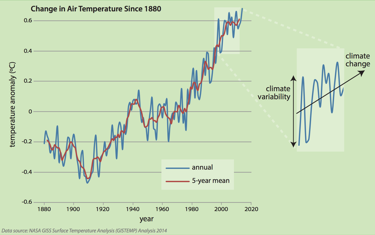
It is therefore important to take this variability into account when analyzing climate data.
Climatology and Anomalies
One common way to do this is to calculate a climatology, which is the average value of a variable over a specific period of time (e.g. 30 years) for a specific location and time of year. This allows us to identify what is normal for a given location and time of year and to calculate anomalies, which are the difference between the observed value and the climatology. These are also referred to as climate normals.
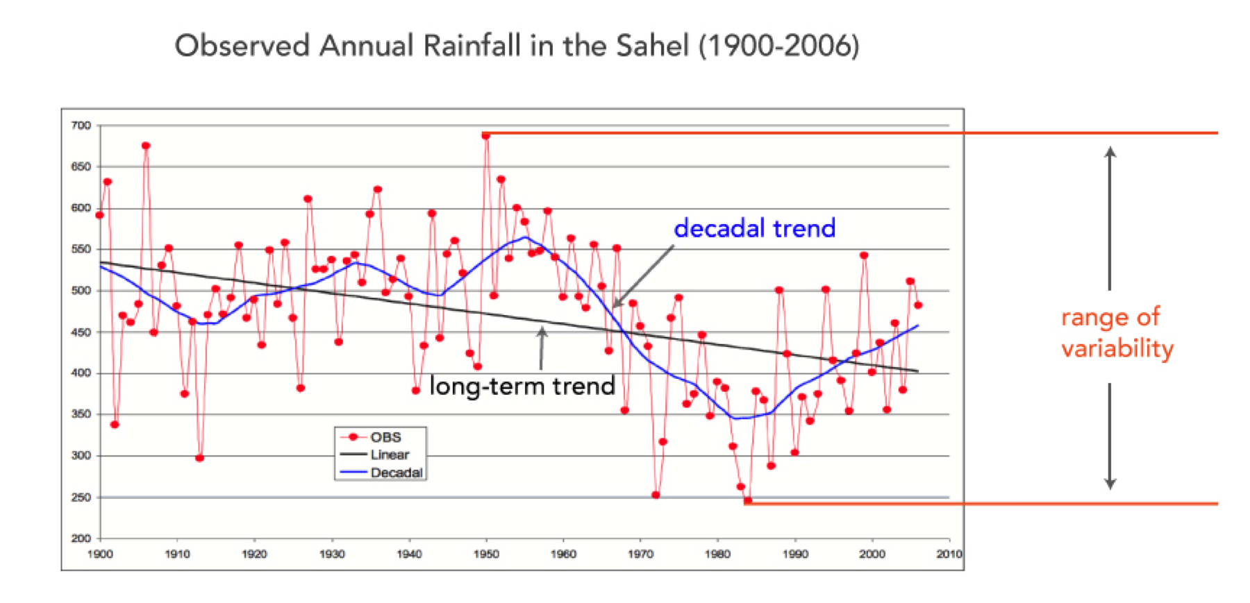
A period of 30-years is commonly used to calculate climatologies, because it is long enough to capture the natural variability of the climate system, but short enough to capture the long-term trends in the data (Figure 3).
We can see in the figure below how the climate has been warming when comparing these 30-year climate averages to the 20th century average (Figure 4).

Rolling Means
Rolling means are another common way to smooth out short-term variability in the data and to identify long-term trends. A rolling mean is calculated by taking the average of a variable over a specific window of time (e.g. 5 years) and then moving that window across the data. This allows us to see the underlying variation in the data without being affected by short-term fluctuations.
ENSO
There are many sources of natural variability in the climate system, which can affect the observed trends in the data. One of the most well-known sources of natural variability is the El Niño Southern Oscillation (ENSO), which is a periodic fluctuation in sea surface temperatures and atmospheric pressure in the equatorial Pacific Ocean. ENSO has a significant impact on global weather and climate patterns, including precipitation, temperature, and storm activity.
El Niño is a so-called teleconnection, which means an atmospheric or oceanic phenomenon that has effects on weather and climate patterns in other parts of the world. For example, El Niño can lead to increased precipitation in the southern United States and drought in Australia and Indonesia.
The El Niño phenomenon stems from an oscillation in circulation system in the pacific, leading to changes in sea surface temperatures and atmospheric pressure. The figure below shows the typical circulation pattern during El Niño conditions (Figure 5).
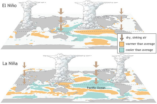
These wind changes cause upwelling of cold water in the eastern Pacific to weaken, which leads to a warming of the ocean surface in the central and eastern tropical Pacific Ocean. This warming of the ocean surface is what we refer to as El Niño.
This means that there are three phases of ENSO (@#fig-enso-sst-anomaly):
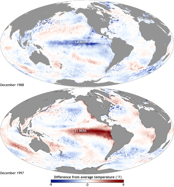
- El Niño: A warming of the ocean surface, or above-average sea surface temperatures (SST), in the central and eastern tropical Pacific Ocean. Over Indonesia, rainfall tends to become reduced while rainfall increases over the tropical Pacific Ocean. The low-level surface winds, which normally blow from east to west along the equator (“easterly winds”), instead weaken or, in some cases, start blowing the other direction (from west to east or “westerly winds”).
- La Niña: A cooling of the ocean surface, or below-average sea surface temperatures (SST), in the central and eastern tropical Pacific Ocean. Over Indonesia, rainfall tends to increase while rainfall decreases over the central tropical Pacific Ocean. The normal easterly winds along the equator become even stronger.
- Neutral: Neither El Niño or La Niña. Often tropical Pacific SSTs are generally close to average. However, there are some instances when the ocean can look like it is in an El Niño or La Niña state, but the atmosphere is not playing along (or vice versa).
Side note:
There have been recent media reports (e.g. here) on the possibility of a “super El Niño” in 2026. Because the El Niño phase of ENSO is associated with transfer of heat from the ocean to the atmosphere such an event would likely lead to a significant short-term increase in global temperatures. In fact, the so-called global warming hiatus occurred when the strong 1998 El Niño was followed by a strong La Niña, which led to the transfer of heat from the atmosphere back into the ocean and a temporary slowdown of global warming.