import pandas as pdWorking with timeseries data
Reading timeseries data: Weather station data
In this example, we will se NOAA weather station data that I downloaded from Climate Data Online. We are using data from Charlottesville-Albemarle Airport. In this particular daily summaries are archived.
We read the data like in previous examples. With no options, this is what we get.
datafile = r'../Data/CDO_USW00093736_1955_2025.txt'
df = pd.read_csv(datafile)
df.head()| STATION ELEVATION LATITUDE LONGITUDE DATE PRCP SNWD SNOW TAVG TMAX TMIN AWND WDF2 WDF5 WSF2 WSF5 | |
|---|---|
| 0 | ----------------- ---------- ---------- ------... |
| 1 | GHCND:USW00093736 194.8 38.14 -7... |
| 2 | GHCND:USW00093736 194.8 38.14 -7... |
| 3 | GHCND:USW00093736 194.8 38.14 -7... |
| 4 | GHCND:USW00093736 194.8 38.14 -7... |
Pandas did not separate the data into different columns. This is because it was expecting a standard csv file with comma separated values. However, in our file the data is separated by multiple whitespaces. We can let pandas know by using the sep keyword. \s indicates a whitespace and the + is for multiple.
We also see that the first row in the dataset does not contain any data. We use the skiprows keyword to indicate that the second-row (1st when counting from zero) does not have any data. As a standard, pandas assumes that the first row contains the column-headers.
df = pd.read_csv(datafile, sep=r'\s+', skiprows= [1])
df.head()| STATION | ELEVATION | LATITUDE | LONGITUDE | DATE | PRCP | SNWD | SNOW | TAVG | TMAX | TMIN | AWND | WDF2 | WDF5 | WSF2 | WSF5 | |
|---|---|---|---|---|---|---|---|---|---|---|---|---|---|---|---|---|
| 0 | GHCND:USW00093736 | 194.8 | 38.14 | -78.45 | 19560101 | -9999.0 | -9999.0 | -9999.0 | -9999.0 | 10.0 | -1.7 | -9999.0 | -9999 | -9999 | -9999.0 | -9999.0 |
| 1 | GHCND:USW00093736 | 194.8 | 38.14 | -78.45 | 19560102 | -9999.0 | -9999.0 | -9999.0 | -9999.0 | 4.4 | -3.9 | -9999.0 | -9999 | -9999 | -9999.0 | -9999.0 |
| 2 | GHCND:USW00093736 | 194.8 | 38.14 | -78.45 | 19560103 | -9999.0 | -9999.0 | -9999.0 | -9999.0 | 12.8 | 0.6 | -9999.0 | -9999 | -9999 | -9999.0 | -9999.0 |
| 3 | GHCND:USW00093736 | 194.8 | 38.14 | -78.45 | 19560104 | -9999.0 | -9999.0 | -9999.0 | -9999.0 | 8.9 | -2.8 | -9999.0 | -9999 | -9999 | -9999.0 | -9999.0 |
| 4 | GHCND:USW00093736 | 194.8 | 38.14 | -78.45 | 19560105 | -9999.0 | -9999.0 | -9999.0 | -9999.0 | 11.7 | 0.0 | -9999.0 | -9999 | -9999 | -9999.0 | -9999.0 |
This looks much better. We also see that there are lots of -9999 and -9999.0 values. The CDO documentation tells us that these are used to identify missing data, so we can let pandas know.
df = pd.read_csv(datafile, sep=r'\s+', skiprows= [1], na_values= [-9999, -9999.0])
df.head()| STATION | ELEVATION | LATITUDE | LONGITUDE | DATE | PRCP | SNWD | SNOW | TAVG | TMAX | TMIN | AWND | WDF2 | WDF5 | WSF2 | WSF5 | |
|---|---|---|---|---|---|---|---|---|---|---|---|---|---|---|---|---|
| 0 | GHCND:USW00093736 | 194.8 | 38.14 | -78.45 | 19560101 | NaN | NaN | NaN | NaN | 10.0 | -1.7 | NaN | NaN | NaN | NaN | NaN |
| 1 | GHCND:USW00093736 | 194.8 | 38.14 | -78.45 | 19560102 | NaN | NaN | NaN | NaN | 4.4 | -3.9 | NaN | NaN | NaN | NaN | NaN |
| 2 | GHCND:USW00093736 | 194.8 | 38.14 | -78.45 | 19560103 | NaN | NaN | NaN | NaN | 12.8 | 0.6 | NaN | NaN | NaN | NaN | NaN |
| 3 | GHCND:USW00093736 | 194.8 | 38.14 | -78.45 | 19560104 | NaN | NaN | NaN | NaN | 8.9 | -2.8 | NaN | NaN | NaN | NaN | NaN |
| 4 | GHCND:USW00093736 | 194.8 | 38.14 | -78.45 | 19560105 | NaN | NaN | NaN | NaN | 11.7 | 0.0 | NaN | NaN | NaN | NaN | NaN |
Great. The missing data is now represented by NaN.
What data types did pandas infer?
df.info()<class 'pandas.DataFrame'>
RangeIndex: 25554 entries, 0 to 25553
Data columns (total 16 columns):
# Column Non-Null Count Dtype
--- ------ -------------- -----
0 STATION 25554 non-null str
1 ELEVATION 25554 non-null float64
2 LATITUDE 25554 non-null float64
3 LONGITUDE 25554 non-null float64
4 DATE 25554 non-null int64
5 PRCP 23343 non-null float64
6 SNWD 5958 non-null float64
7 SNOW 5970 non-null float64
8 TAVG 2831 non-null float64
9 TMAX 25498 non-null float64
10 TMIN 25496 non-null float64
11 AWND 9914 non-null float64
12 WDF2 9919 non-null float64
13 WDF5 9899 non-null float64
14 WSF2 9920 non-null float64
15 WSF5 9901 non-null float64
dtypes: float64(14), int64(1), str(1)
memory usage: 3.5 MBDo you notice a problem. The DATE column was read as an integer, which means that pandas did not understand that this is a date.
So, January 1st 1956 became 19560101
We need to explicitly tell pandas, which columns should be understood as dates:
df = pd.read_csv(datafile, sep=r'\s+',
                 na_values=[-9999.0, -99.0],
                 skiprows = [1],
                 parse_dates=[4])
df.info()
<class 'pandas.DataFrame'>
RangeIndex: 25554 entries, 0 to 25553
Data columns (total 16 columns):
# Column Non-Null Count Dtype
--- ------ -------------- -----
0 STATION 25554 non-null str
1 ELEVATION 25554 non-null float64
2 LATITUDE 25554 non-null float64
3 LONGITUDE 25554 non-null float64
4 DATE 25554 non-null datetime64[us]
5 PRCP 23343 non-null float64
6 SNWD 5958 non-null float64
7 SNOW 5970 non-null float64
8 TAVG 2831 non-null float64
9 TMAX 25498 non-null float64
10 TMIN 25496 non-null float64
11 AWND 9914 non-null float64
12 WDF2 9919 non-null float64
13 WDF5 9899 non-null float64
14 WSF2 9920 non-null float64
15 WSF5 9901 non-null float64
dtypes: datetime64[us](1), float64(14), str(1)
memory usage: 3.5 MBThat worked.
Time indices
Indexes are very powerful. They are a big part of why Pandas is so useful. There are different indices for different types of data. Time Indexes are especially great!
We now set the date column as the index for our dataframe.
df = df.set_index('DATE')
df.head()| STATION | ELEVATION | LATITUDE | LONGITUDE | PRCP | SNWD | SNOW | TAVG | TMAX | TMIN | AWND | WDF2 | WDF5 | WSF2 | WSF5 | |
|---|---|---|---|---|---|---|---|---|---|---|---|---|---|---|---|
| DATE | |||||||||||||||
| 1956-01-01 | GHCND:USW00093736 | 194.8 | 38.14 | -78.45 | NaN | NaN | NaN | NaN | 10.0 | -1.7 | NaN | NaN | NaN | NaN | NaN |
| 1956-01-02 | GHCND:USW00093736 | 194.8 | 38.14 | -78.45 | NaN | NaN | NaN | NaN | 4.4 | -3.9 | NaN | NaN | NaN | NaN | NaN |
| 1956-01-03 | GHCND:USW00093736 | 194.8 | 38.14 | -78.45 | NaN | NaN | NaN | NaN | 12.8 | 0.6 | NaN | NaN | NaN | NaN | NaN |
| 1956-01-04 | GHCND:USW00093736 | 194.8 | 38.14 | -78.45 | NaN | NaN | NaN | NaN | 8.9 | -2.8 | NaN | NaN | NaN | NaN | NaN |
| 1956-01-05 | GHCND:USW00093736 | 194.8 | 38.14 | -78.45 | NaN | NaN | NaN | NaN | 11.7 | 0.0 | NaN | NaN | NaN | NaN | NaN |
The TimeIndex object has lots of useful attributes. Below are some examples:
df.index.monthIndex([1, 1, 1, 1, 1, 1, 1, 1, 1, 1,
...
2, 2, 2, 2, 2, 2, 2, 2, 2, 2],
dtype='int32', name='DATE', length=25554)df.index.yearIndex([1956, 1956, 1956, 1956, 1956, 1956, 1956, 1956, 1956, 1956,
...
2026, 2026, 2026, 2026, 2026, 2026, 2026, 2026, 2026, 2026],
dtype='int32', name='DATE', length=25554)df.index.day_of_weekIndex([6, 0, 1, 2, 3, 4, 5, 6, 0, 1,
...
2, 3, 4, 5, 6, 0, 1, 2, 3, 4],
dtype='int32', name='DATE', length=25554)We can also use the time index to calculate the length of a period.
df.index[10] - df.index[0] Timedelta('10 days 00:00:00')(df.index[10] - df.index[0]).total_seconds() 864000.0Accessing data through the time index
We can now access values by time:
df.loc['2017-08-07']STATION GHCND:USW00093736
ELEVATION 192.3
LATITUDE 38.1374
LONGITUDE -78.45513
PRCP 26.7
SNWD NaN
SNOW NaN
TAVG NaN
TMAX 25.6
TMIN 21.1
AWND 1.5
WDF2 30.0
WDF5 320.0
WSF2 5.8
WSF5 7.2
Name: 2017-08-07 00:00:00, dtype: objectOr use slicing to get a range:
df.loc['2017-07-01':'2017-07-31']| STATION | ELEVATION | LATITUDE | LONGITUDE | PRCP | SNWD | SNOW | TAVG | TMAX | TMIN | AWND | WDF2 | WDF5 | WSF2 | WSF5 | |
|---|---|---|---|---|---|---|---|---|---|---|---|---|---|---|---|
| DATE | |||||||||||||||
| 2017-07-01 | GHCND:USW00093736 | 192.3 | 38.1374 | -78.45513 | 0.0 | NaN | NaN | NaN | 34.4 | 23.3 | 2.7 | 190.0 | 120.0 | 6.7 | 8.9 |
| 2017-07-02 | GHCND:USW00093736 | 192.3 | 38.1374 | -78.45513 | 0.0 | NaN | NaN | NaN | 31.7 | 20.6 | 1.5 | 200.0 | 210.0 | 5.8 | 8.1 |
| 2017-07-03 | GHCND:USW00093736 | 192.3 | 38.1374 | -78.45513 | 0.0 | NaN | NaN | NaN | 33.9 | 19.4 | 0.9 | 210.0 | 210.0 | 5.4 | 6.3 |
| 2017-07-04 | GHCND:USW00093736 | 192.3 | 38.1374 | -78.45513 | 0.3 | NaN | NaN | NaN | 32.2 | 21.1 | 0.8 | 210.0 | 200.0 | 4.0 | 5.4 |
| 2017-07-05 | GHCND:USW00093736 | 192.3 | 38.1374 | -78.45513 | 5.3 | NaN | NaN | NaN | 27.8 | 22.2 | 2.0 | 80.0 | 60.0 | 6.3 | 8.1 |
| 2017-07-06 | GHCND:USW00093736 | 192.3 | 38.1374 | -78.45513 | 0.5 | NaN | NaN | NaN | 31.7 | 21.7 | 1.3 | 210.0 | 60.0 | 5.8 | 6.7 |
| 2017-07-07 | GHCND:USW00093736 | 192.3 | 38.1374 | -78.45513 | 0.0 | NaN | NaN | NaN | 33.3 | 22.8 | 1.7 | 200.0 | 210.0 | 5.8 | 8.5 |
| 2017-07-08 | GHCND:USW00093736 | 192.3 | 38.1374 | -78.45513 | 0.0 | NaN | NaN | NaN | 32.8 | 20.0 | 1.6 | 320.0 | 330.0 | 5.8 | 8.1 |
| 2017-07-09 | GHCND:USW00093736 | 192.3 | 38.1374 | -78.45513 | 0.0 | NaN | NaN | NaN | 31.1 | 17.2 | 0.9 | 160.0 | 160.0 | 5.4 | 6.3 |
| 2017-07-10 | GHCND:USW00093736 | 192.3 | 38.1374 | -78.45513 | 0.0 | NaN | NaN | NaN | 33.9 | 17.2 | 2.0 | 190.0 | 190.0 | 6.7 | 9.4 |
| 2017-07-11 | GHCND:USW00093736 | 192.3 | 38.1374 | -78.45513 | 0.0 | NaN | NaN | NaN | 31.1 | 20.6 | 2.2 | 200.0 | 190.0 | 5.8 | 7.2 |
| 2017-07-12 | GHCND:USW00093736 | 192.3 | 38.1374 | -78.45513 | 0.0 | NaN | NaN | NaN | 36.1 | 22.8 | 1.6 | 260.0 | 260.0 | 5.4 | 6.7 |
| 2017-07-13 | GHCND:USW00093736 | 192.3 | 38.1374 | -78.45513 | 0.5 | NaN | NaN | NaN | 36.7 | 22.8 | 2.0 | 230.0 | 210.0 | 7.2 | 9.4 |
| 2017-07-14 | GHCND:USW00093736 | 192.3 | 38.1374 | -78.45513 | 22.6 | NaN | NaN | NaN | 37.8 | 23.9 | 2.3 | 340.0 | 320.0 | 10.3 | 17.0 |
| 2017-07-15 | GHCND:USW00093736 | 192.3 | 38.1374 | -78.45513 | 0.0 | NaN | NaN | NaN | 33.3 | 22.8 | 1.6 | 340.0 | 340.0 | 4.5 | 6.7 |
| 2017-07-16 | GHCND:USW00093736 | 192.3 | 38.1374 | -78.45513 | 0.0 | NaN | NaN | NaN | 32.8 | 20.6 | 1.5 | 120.0 | 140.0 | 4.0 | 6.3 |
| 2017-07-17 | GHCND:USW00093736 | 192.3 | 38.1374 | -78.45513 | 0.0 | NaN | NaN | NaN | 32.8 | 20.6 | 1.4 | 170.0 | 180.0 | 7.6 | 9.4 |
| 2017-07-18 | GHCND:USW00093736 | 192.3 | 38.1374 | -78.45513 | 0.0 | NaN | NaN | NaN | 35.0 | 20.0 | 1.5 | 150.0 | 150.0 | 7.6 | 10.3 |
| 2017-07-19 | GHCND:USW00093736 | 192.3 | 38.1374 | -78.45513 | 0.0 | NaN | NaN | NaN | 35.6 | 18.9 | 0.9 | 100.0 | 350.0 | 4.0 | 5.4 |
| 2017-07-20 | GHCND:USW00093736 | 192.3 | 38.1374 | -78.45513 | 0.0 | NaN | NaN | NaN | 36.7 | 21.7 | 1.2 | 190.0 | 290.0 | 5.8 | 8.9 |
| 2017-07-21 | GHCND:USW00093736 | 192.3 | 38.1374 | -78.45513 | 5.8 | NaN | NaN | NaN | 36.7 | 23.3 | 1.1 | 320.0 | 310.0 | 8.9 | 14.8 |
| 2017-07-22 | GHCND:USW00093736 | 192.3 | 38.1374 | -78.45513 | 1.3 | NaN | NaN | NaN | 36.7 | 22.8 | 2.1 | 50.0 | 350.0 | 7.6 | 10.3 |
| 2017-07-23 | GHCND:USW00093736 | 192.3 | 38.1374 | -78.45513 | 0.0 | NaN | NaN | NaN | 34.4 | 23.3 | 1.5 | 200.0 | 190.0 | 9.4 | 13.0 |
| 2017-07-24 | GHCND:USW00093736 | 192.3 | 38.1374 | -78.45513 | 9.4 | NaN | NaN | NaN | 33.3 | 22.8 | 2.6 | 190.0 | 160.0 | 11.6 | 14.3 |
| 2017-07-25 | GHCND:USW00093736 | 192.3 | 38.1374 | -78.45513 | 0.0 | NaN | NaN | NaN | 30.0 | 18.9 | 2.7 | 20.0 | 40.0 | 6.7 | 8.5 |
| 2017-07-26 | GHCND:USW00093736 | 192.3 | 38.1374 | -78.45513 | 0.0 | NaN | NaN | NaN | 30.0 | 16.7 | 1.0 | 200.0 | 180.0 | 5.4 | 7.6 |
| 2017-07-27 | GHCND:USW00093736 | 192.3 | 38.1374 | -78.45513 | 0.5 | NaN | NaN | NaN | 31.1 | 20.0 | 1.4 | 210.0 | 190.0 | 5.4 | 6.7 |
| 2017-07-28 | GHCND:USW00093736 | 192.3 | 38.1374 | -78.45513 | 51.1 | NaN | NaN | NaN | 30.0 | 22.2 | 1.2 | 210.0 | 200.0 | 5.4 | 6.3 |
| 2017-07-29 | GHCND:USW00093736 | 192.3 | 38.1374 | -78.45513 | 0.3 | NaN | NaN | NaN | 26.7 | 17.2 | 3.8 | 40.0 | 20.0 | 10.3 | 12.5 |
| 2017-07-30 | GHCND:USW00093736 | 192.3 | 38.1374 | -78.45513 | 0.0 | NaN | NaN | NaN | 28.9 | 13.3 | 1.3 | 30.0 | 50.0 | 5.4 | 6.7 |
| 2017-07-31 | GHCND:USW00093736 | 192.3 | 38.1374 | -78.45513 | 0.0 | NaN | NaN | NaN | 31.1 | 15.0 | 0.8 | 70.0 | 90.0 | 4.5 | 5.8 |
Plotting data
Pandas is very “time aware” and will format the axis of our plot accordingly.
df.loc['2017-01-01':'2017-12-31', 'TMAX'].plot()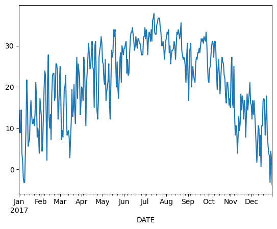
Aggregating data
This timeseries has daily resolution, and the daily plots can be very noisy.
df.plot(y='TMAX') 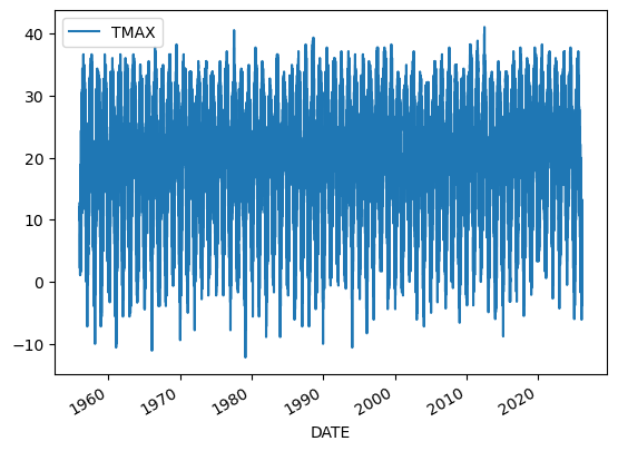
Aggregating our data will help us reduce the noise.
Resampling data
A common operation is to change the resolution of a dataset by resampling in time. Pandas exposes this through the resample function. The resample periods are specified using pandas offset index syntax.
Below we resample the dataset by getting the data for every year. YS stands for year start. A full list of these so-called offset aliases is found in the pandas timeseries documentation.
yearly_df=df[['TMIN', 'TMAX']].resample('YS').mean()
yearly_df.head()| TMIN | TMAX | |
|---|---|---|
| DATE | ||
| 1956-01-01 | 9.924501 | 19.512821 |
| 1957-01-01 | 10.489779 | 19.036464 |
| 1958-01-01 | 8.379614 | 17.766391 |
| 1959-01-01 | 9.181096 | 19.614247 |
| 1960-01-01 | 8.561749 | 18.340984 |
yearly_df.plot()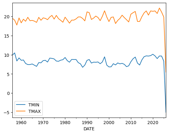
This looks much less noisy, and we could for example now think about whether there is a trend in our dataset.
Groupby
We have already seen how powerful the .groupby() operation is.
A common way to analyze weather data in climate science is to create a “climatology,” which contains the average values in each month or day of the year. We can do this easily with .groupby(). Recall that df.index is a pandas DateTimeIndex object.
monthly_climatology  = df[['TMIN', 'TMAX']].groupby(df.index.month).mean()
monthly_climatology | TMIN | TMAX | |
|---|---|---|
| DATE | ||
| 1 | -2.707156 | 7.235597 |
| 2 | -1.510136 | 9.175895 |
| 3 | 2.457680 | 14.229545 |
| 4 | 7.643440 | 20.404322 |
| 5 | 12.485556 | 24.526753 |
| 6 | 17.079532 | 28.774678 |
| 7 | 19.510906 | 30.701017 |
| 8 | 18.657407 | 29.771930 |
| 9 | 14.877751 | 26.253037 |
| 10 | 8.311281 | 20.599676 |
| 11 | 3.371483 | 14.821412 |
| 12 | -0.699630 | 9.224699 |
Each row in this new dataframe respresents the average values for the months (1=January, 2=February, etc.)
We can apply more customized aggregations. These can be specified using .aggregate(). Below we keep the max of the TMAX column, and min of TMIN column for the temperature measurements.
monthly_T_climatology = df.groupby(df.index.month).aggregate({'TMAX': 'max',
                                                              'TMIN': 'min'})
monthly_T_climatology.head()| TMAX | TMIN | |
|---|---|---|
| DATE | ||
| 1 | 27.2 | -21.1 |
| 2 | 27.8 | -19.4 |
| 3 | 32.8 | -17.1 |
| 4 | 34.4 | -5.6 |
| 5 | 36.1 | -1.7 |
monthly_T_climatology.plot(marker='o')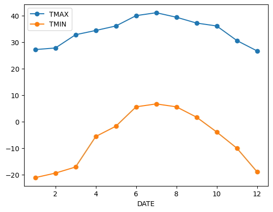
If we want to do it on a finer scale, we can group by day of year
daily_T_climatology = df.groupby(df.index.dayofyear).aggregate({'TMAX': 'max',
                                                              'TMIN': 'min'})
daily_T_climatology.plot(marker='.')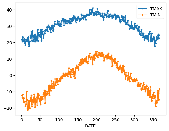
Missing data and gapfilling
Because timeseries data is ordered and can show periodic variation (e.g. seasonal, daily, annual) dealing with missing data is very important.
Take precipitation data for example.
df['PRCP'].plot(kind='hist',ylabel='Frequency', xlabel='Precipitation (mm)', bins=20, grid = True)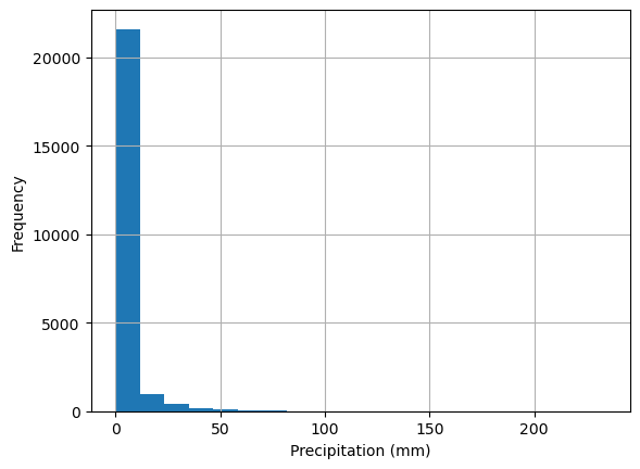
Because rainfall is intermittent and the majority of days are dry, rainfall is typically reported as annual or monthly Let’s look at the period between 1980 and 2000.
df_20_years = df.loc['1980':'2000']
df_20_years.groupby(df_20_years.index.year)['PRCP'].sum().plot(kind='bar',xlabel='Year', ylabel='Total Precipitation (mm)', title='Total Precipitation by Year (1980-2000)') 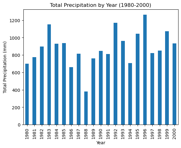
Using the data as is, it appears that 1988 and 1994 were unusually dry.
We can check the same period for missing data. The .isna() method returns True when data is missing (i.e. NaN). We can also use the feature that True is counted as 1 and False as 0.
So the below code, produces a series with True for missing days and False for days with data. The Trues are then summed up.
df_20_years['PRCP'].isna().groupby(df_20_years.index.year).sum().plot(grid=True, ylabel='Number of Missing Days', title='Missing Data by Year (1980-2000)')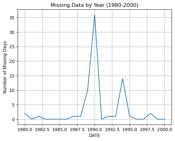
Pandas has built in methods for filling in missing data. The simplest is to fill in a constant value, such as the mean, median, or zero.
For example, we can fill in missing precipitation values with the average rainfall
df_20_years['PRCP'].mean()np.float64(2.4337458854509544)df_20_years_filled = df_20_years['PRCP'].fillna(df_20_years['PRCP'].mean())
df_20_years_filled.groupby(df_20_years_filled.index.year).sum().plot(kind='bar',xlabel='Year', ylabel='Total Precipitation (mm)', title='Total Precipitation by Year (1980-2000) Gapfilled with Mean') 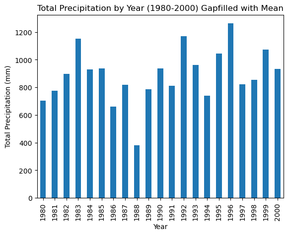
This did not change the result much. Gapfilling is difficult without knowing the dataset very well. For example, the missing data in 1998 could have missed by chance some of the largest rainshowers of the year so that adding the average rainfall makes little different.
Pandas offers several ways of dealing with missing data.
- Interpolation:
df.interpolate(method = 'linear', ...)fillsNaNvalues using an interpolation method. There are several methods available includinglinear,splines, … - Forward fill:
df.ffill()fillsNaNvalues by propagating the last valid observation to next valid. - Backward fill:
df.bfill() - Remove rows with NaN:
df.dropna()simply removes any rows that containNaNvalues. This is not recommended for time series data.
In reality each of these methods will only work for small numbers of missing data.