import pandas as pd
import matplotlib.pyplot as plt
from scipy.stats import pearson3Flood return period and probability
In this lesson, we use streamflow data from a USGS stream gauge at the South River Near Waynesboro.
At this location daily stream discharge (i.e. the total volume of water in \(ft^3/s\)) has been reported since 1952. The data was downloaded using the USGS Water data API and we will discuss what APIs are later in the course.
For today, the goal is to process the data in a way that we can estimate the probabilities of a different magnitude events of river discharge.
Learning goals
- Calculate exceedance probability and return periods associated with a flood in Python.
- Use statistical tools to fit a statistical distribution for flood probability to the data
- Predict river discharge return rates outside the observed range (e.g. the probability of a 100-year or 200-year flood)
- Understand limitations of this approach
We first load the libraries that we will need. In addition to pandas, matplotlib.pyplot and numpy, we will also use the scipy.stats statistics package to fit our model.
Loading the data
We are now reading the data. This is similar to the previous weeks. The only difference is that I am removing the time-zone information from the data, which makes the time display less cluttered.
df = pd.read_csv('../Data/usgs_nwis_01626000_1952-10-01.csv',
                 parse_dates=[0],
                 na_values=[-999999])
df.datetime = pd.to_datetime(df.datetime).dt.tz_localize(None) # removes the time-zone information
df = df.set_index('datetime')
df.head()| site_no | 00060_Mean | 00060_Mean_cd | |
|---|---|---|---|
| datetime | |||
| 1952-10-01 | 1626000 | 38.0 | A |
| 1952-10-02 | 1626000 | 39.0 | A |
| 1952-10-03 | 1626000 | 39.0 | A |
| 1952-10-04 | 1626000 | 38.0 | A |
| 1952-10-05 | 1626000 | 38.0 | A |
We can see that we have a time series. The 00060_Mean column contains the average daily discharge in \(ft^3/s\). This can be looked up in the API documentation which specifies the variable code 60 for streamflow. What does the 00060_Mean_cd mean?
Let’s have a look.
Exploring the data
df['00060_Mean_cd'].value_counts()00060_Mean 00060_Mean_cd
35.0 A 308
38.0 A 297
36.0 A 295
34.0 A 290
31.0 A 290
...
42.5 P 1
65.4 P 1
63.9 P 1
141.0 P 1
162.0 P 1
Name: count, Length: 2381, dtype: int64Without context this does not make much sense. From the API documentation we can learn that A and P are codes for approved and provisional. e stands for estimated and Ice is an observation code for the presence of ice which will affect water quality.
In a real-world analysis, we should think about what this would mean for our analysis. For now we are OK with the data as is.
Let’s make our data a bit easier and only keep the discharge. I am also renaming that column using .rename().
colunms_to_keep = ['00060_Mean']
df = df[colunms_to_keep]
df = df.rename(columns={'00060_Mean': 'discharge'})
df.head() | discharge | |
|---|---|
| datetime | |
| 1952-10-01 | 38.0 |
| 1952-10-02 | 39.0 |
| 1952-10-03 | 39.0 |
| 1952-10-04 | 38.0 |
| 1952-10-05 | 38.0 |
We look at some basic statistics.
df.describe()| discharge | |
|---|---|
| count | 26802.000000 |
| mean | 149.751936 |
| std | 263.541643 |
| min | 15.700000 |
| 25% | 44.000000 |
| 50% | 83.000000 |
| 75% | 164.000000 |
| max | 9670.000000 |
From these we can already see that the data is pretty skewed. Most days there are moderate to low streamflows, but there are large extremes. The behavior of these extremes is what we want to model.
Let’s plot our data to understand this better.
df['discharge'].plot(kind='line', ylabel= 'streamflow (cfs)', title='Daily mean streamflow at USGS 01626000', xlabel='Date')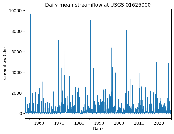
This confirms our previous analysis. We can see these “spikes” of high streamflow.
Calculating Annual Maxima
Since we are interested flood probability, we can simplify our data further by only retaining the annual maxima.
df_annual_max = df.resample('YS').max()
df_annual_max.head()| discharge | |
|---|---|
| datetime | |
| 1952-01-01 | 950.0 |
| 1953-01-01 | 1540.0 |
| 1954-01-01 | 1000.0 |
| 1955-01-01 | 9670.0 |
| 1956-01-01 | 1960.0 |
We can create a histogram to better understand the distribution of the annual maximum streamflow.
fig, ax = plt.subplots()
df_annual_max.plot(kind='hist', y = 'discharge', bins = 20, ax = ax)
ax.set_xlabel('Annual maximum streamflow (cfs)')
ax.set_title('Histogram of annual maximum streamflow at USGS 01626000')
Text(0.5, 1.0, 'Histogram of annual maximum streamflow at USGS 01626000')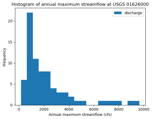
The histogram reveals a distribution with strong right-skew. This is very different from temperature and other data that you have encountered before, which is much closer to a normal distribution.
Calculating flood event probabilities
We are now ready to calculate the flood event return probability from the data. There are several ways to do this, that assume differences in the underlying distribution of the data.
Here we want to calculate the probability for a flood event to exceed a certain threshold. Statistically speaking the Exceedance Probability is related to a Cumulative distribution function (CDF), which describes the probability that an event will take a value of less then a certain value.
The figure below shows an empirical CDF.

\(\text{Exceedance Probability} = 1-CDF(x)\)
One way of deriving this is to calculate a simple Rank-oder probability as:
\(\text{Exceedance Probability} = \frac{n-i+1}{n+1}\)
where \(i\) is the rank order (smallest to largest) from 1 to \(n\). Note that the limits of this equation vary from \(n/(n+1)\) ~ 1 for the smallest events and \(1/(n+1)\) for the largest events (i.e., the largest events have a very small exceedance probability).
Therefore we implement the following steps:
- Sort the data from smallest to largest.
- Calculate exceedance probabilities using the equation below where
nis length of the record andiis the rank. - Calculate the inverse of the exceedance probabilities to determine return period in years.
This is implemented in the code below using .sort_values() to sort the dataframe and .insert() to create a new column named ['rank'] ranging from \(1\) to \(n\).
sorted_data = df_annual_max.sort_values(by = 'discharge')
n = len(sorted_data) # number of data points
sorted_data.insert(0, 'rank', range(1, 1 + n)) # insert rank column
sorted_data['probability'] = (n - sorted_data["rank"] + 1) / (n + 1) # calculate probability
sorted_data['return_years'] = 1/sorted_data['probability'] # calculate return years
sorted_data| rank | discharge | probability | return_years | |
|---|---|---|---|---|
| datetime | ||||
| 2026-01-01 | 1 | 165.0 | 0.986842 | 1.013333 |
| 1981-01-01 | 2 | 312.0 | 0.973684 | 1.027027 |
| 2002-01-01 | 3 | 464.0 | 0.960526 | 1.041096 |
| 2008-01-01 | 4 | 483.0 | 0.947368 | 1.055556 |
| 2000-01-01 | 5 | 556.0 | 0.934211 | 1.070423 |
| ... | ... | ... | ... | ... |
| 1969-01-01 | 71 | 7100.0 | 0.065789 | 15.200000 |
| 1972-01-01 | 72 | 7430.0 | 0.052632 | 19.000000 |
| 2003-01-01 | 73 | 8110.0 | 0.039474 | 25.333333 |
| 1985-01-01 | 74 | 9070.0 | 0.026316 | 38.000000 |
| 1955-01-01 | 75 | 9670.0 | 0.013158 | 76.000000 |
75 rows × 4 columns
We can now plot the streamflow against the annual exceedance probability. In this case, it also makes sense to use a log-scale for the y-axis
sorted_data.plot(kind='scatter',x='discharge', y='probability',logy=True,
                 ylabel='Annual exceedance probability (1/y)',
                 xlabel='Annual maximum streamflow (cfs)',
                 grid = True)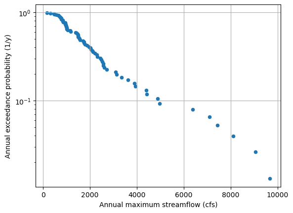
Or we can plot the return-period against the streamflow. We can see that this produces a curve that appears to level off which larger streamflows.
sorted_data.plot(kind='scatter',y='discharge', x='return_years', grid = True,
                 xlabel='Return period (years)',
                 ylabel='Annual maximum streamflow (cfs)')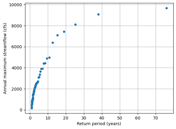
Fitting a statistical model for the return period.
USGS technical guidelines state that streamflow frequencies should be determined by fitting a log-Pearson-III distribution. (Don’t worry if you have never heard about this.)
In response there are several manuals, that provide detailed procedures on how to fit such a distribution to data (example: Texas Department of Transportation Hydraulic Design Manual).
Instead of implementing such a procedure, we will be making use of the python’s statistical tools in the scipy.stats package to perform the fit.
Because scipy.stats only has the Person-Type 3 (Pearson3) distribution, we will do a log-transform on the data.
import numpy as np
sorted_data['log_discharge'] = np.log10(sorted_data['discharge'])

sorted_data.head()| rank | discharge | probability | return_years | log_discharge | |
|---|---|---|---|---|---|
| datetime | |||||
| 2026-01-01 | 1 | 165.0 | 0.986842 | 1.013333 | 2.217484 |
| 1981-01-01 | 2 | 312.0 | 0.973684 | 1.027027 | 2.494155 |
| 2002-01-01 | 3 | 464.0 | 0.960526 | 1.041096 | 2.666518 |
| 2008-01-01 | 4 | 483.0 | 0.947368 | 1.055556 | 2.683947 |
| 2000-01-01 | 5 | 556.0 | 0.934211 | 1.070423 | 2.745075 |
The Pearson3 distribution is defined by 3 parameters (location, scale, and shape/skewness), that can be estimated using scipy.stats.person3.fit().
from scipy.stats import pearson3
skew, loc, scale = pearson3.fit(sorted_data['log_discharge'])
print(skew, loc, scale)
0.07705260123416785 3.2140237605029798 0.3451237739859282We can now use these parameters to estimate the relationship between discharge and probabilities calculated from the P3 distribution.
For example, we can get the modeled probabilities for the observed discharge values.
To do so, we can make use of the fact that the scipi.stats.pearson3 can be used to generate the CDF.
Recall the relationship between Exceedance Probability and CDF: \(P = 1- CDF\)
sorted_data['p_logPearson3']=(1-pearson3.cdf(sorted_data['log_discharge'], skew, loc, scale))
sorted_data| rank | discharge | probability | return_years | log_discharge | p_logPearson3 | |
|---|---|---|---|---|---|---|
| datetime | ||||||
| 2026-01-01 | 1 | 165.0 | 0.986842 | 1.013333 | 2.217484 | 0.998601 |
| 1981-01-01 | 2 | 312.0 | 0.973684 | 1.027027 | 2.494155 | 0.983478 |
| 2002-01-01 | 3 | 464.0 | 0.960526 | 1.041096 | 2.666518 | 0.945975 |
| 2008-01-01 | 4 | 483.0 | 0.947368 | 1.055556 | 2.683947 | 0.939953 |
| 2000-01-01 | 5 | 556.0 | 0.934211 | 1.070423 | 2.745075 | 0.914711 |
| ... | ... | ... | ... | ... | ... | ... |
| 1969-01-01 | 71 | 7100.0 | 0.065789 | 15.200000 | 3.851258 | 0.034600 |
| 1972-01-01 | 72 | 7430.0 | 0.052632 | 19.000000 | 3.870989 | 0.030625 |
| 2003-01-01 | 73 | 8110.0 | 0.039474 | 25.333333 | 3.909021 | 0.024039 |
| 1985-01-01 | 74 | 9070.0 | 0.026316 | 38.000000 | 3.957607 | 0.017411 |
| 1955-01-01 | 75 | 9670.0 | 0.013158 | 76.000000 | 3.985426 | 0.014379 |
75 rows × 6 columns
scipi.stats.pearson3 also provides a method to convert probabilities into discharge values.
To do so, we generate a set of return years that we convert to probabilities. We then use the inverse of the modeled P3 distribution to get predict the log of the modeled discharge.
return_years = np.arange(1,500,1)
log_modeled_discharge = pearson3.isf(1/return_years, skew, loc, scale)
modeled_discharge = 10**(log_modeled_discharge)
We can now plot this.
fix, ax = plt.subplots()
sorted_data.plot(kind='scatter',y='discharge', x='return_years', grid = True, ax=ax)

ax.plot(return_years, modeled_discharge, 'r--')

plt.legend(['Observed', 'Pearson Type III'])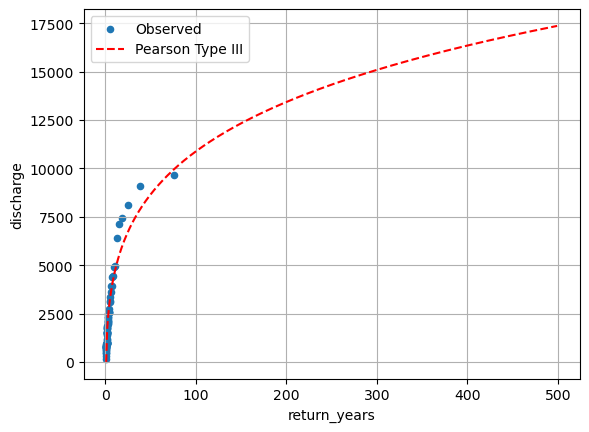
Model Evaluation
We notice that the fit for the extreme values is not particularly good.
One thing that we have not done, and that would typically be absolutely essential is to get a measure of the uncertainty associated with the fitted distribution. The P3-fit does not provide a direct way for quantifying the uncertainty. However, there are methods of generating a confidence interval from the data (e.g. bootstrapping).
There are several reasons, why the model fit may be poor
- Small changes in model parameters will disproportionally affect modeled extreme values
- Extreme events are rare such that parameter fitting that provides an equal weight to all events might discount them
- The Pearson3 distribution might not be the best model
- Not all events are from the same distribution. For example, changes to the river or the climate might have led to a shift in the relationship.
- We deviated from the official and tested fitting procedures
Testing another distribution
The Gumbel Distribution is also frequently used for river discharge modeling.
The Gumbel Probability Distribution is defined as
\(p = e^{-e^{-(x-u)/\alpha}}\)
with
\(u = \bar{x} - 0.577 \alpha\)
\(\alpha = \sqrt{6}\,\frac{\sigma_x}{\pi}\)
\(\bar{x}\) and \(\sigma_x\) are the mean and standard deviations of the observed distribution.
Practice
See whether you can fit a Gumbel distribution to the discharge data. See whether this distribution is a better fit.
Numpy as the exponential function and the square root as: np.exp(), np.sqrt().
This could then be implemented as a function in Python.
def estimate_gumbel(discharge):
    p = ... # code to estimate the parameters of the Gumbel distribution
    return p