Working with Gridded netCDF data and xarray

This lesson is based on the Lesson: working with netCDF data in Fabien Maussion’s Physics of the Climate System Course.

These lecture notes and exercises are licensed under a Creative Commons Attribution 4.0 International (CC BY 4.0) license.

You already learned how to use the basic features of the python language with the numpy and matplotlib libraries. The purpose of this lesson is to introduce you to the main tool that you will use for working with gridded data: xarray.

This is a dense lesson. Please do it entirely and try to remember its structure and content. This code will provide a template for your own code, and you can always come back to these examples when you’ll need them. I don’t expect you to understand all details, but I hope that you are going to get acquainted with the “xarray way” of manipulating multi-dimensional data. You will have to copy and adapt parts of the code below to complete the exercises.

Learning Objectives

Describe netCDF files as self-describing data
Understand how netCDF can be applied to big data
Load netCDF datasets
Select data by time and coordinates
Perform aggregation operations
Plot variables

NetCDF Files

In order to open and plot NetCDF files, you’ll need to install the xarray, cartopy, and netcdf4 packages: if you haven’t done so already, follow the installation instructions for our ISAT420 python environment that contains these packages.

As a quick fix, you can also install them directly using the code below (this will take some time).

#To install these packages remove the hash (#) characters in the lines below and run the cell. The ! tells jupyter to run a system command. 
#! conda install xarray
#! conda install netcdf4
#! conda install cartopy

Imports and options

First, let’s import the tools we need. Remember why we need to import our tools? If not, ask Dr. Gerken

# Import the tools we are going to need today:
import matplotlib.pyplot as plt  # plotting library
import numpy as np  # numerical library
import xarray as xr  # netCDF library
import cartopy  # Map projections libary
import cartopy.crs as ccrs  # Projections list
from glob import glob
# Some defaults:
plt.rcParams['figure.figsize'] = (12, 5)  # Default plot size

The Data

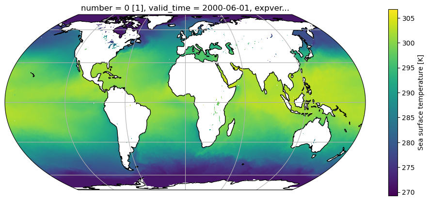
We will also be using an example of ERA5 Reanalysis data.

ERA5 (or European ReAnalysis v5) provides global, hourly estimates of atmospheric, ocean wave, and land-surface variables at a horizontal resolution of 31,km. Data is available from 1940 onwards both hourly and averaged to monthly.

Reanalysis in general are the fusion of observations with a global weather model to derive a homogenous, regular-best estimate output on a grid from station based observations.

ERA5 is produced by the European Center for Medium Range Weather Forecasting (ECMWF) and can be downloaded freely (account registration required).

I have placed the data files into the W8_Xarray_Gridded/Data directory.

Read the data

Most of today’s meteorological data is stored in the NetCDF format (*.nc). NetCDF files are binary files, which means that you can’t just open them in a text editor. You need a special reader for it. Nearly all the programming languages offer an interface to NetCDF. For this course we are going to use the xarray library to read the data:

Xarray commands are similar to pandas but not quite the same. To open a dataset ds we can use the .open_dataset() method.

Let’s start with having a look at the ERA5 file, I am providing.

# Here I downloaded the file in the "Data" folder which I placed in a folder close to this notebook
# The variable name "ds" stands for "dataset"
ds = xr.open_dataset(r'../data/reanalysis-era5-single-level-monthly-means_2000_T_Td_u_v_SST.nc', engine='netcdf4')

# Lets see what we have:
ds

Each netcdf file has a data model, that is represented by xarray:

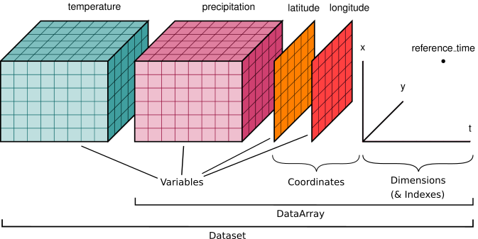
The NetCDF dataset is made up of various elements: Dimensions, Coordinates, Variables, Attributes:

the dimensions specify the number of elements of each data coordinate, their names should be understandable and specific
the attributes provide some information about the file (metadata)
the variables contain the actual data. In our file there are five variables. All have the dimensions [time, latitude, longitude], so we can expect an array of size [12, 721, 1440]
the coordinates locate the data in space and time

Working with big data

The entire ERA5 dataset is larger than 5 Petabytes. This is 5,000,000 GB. Your laptop has 8-16 GB of working memory (RAM) and even supercomputers cannot access more than a few TB of RAM.

Lazy execution

When loading a dataset in Pandas, you are always reading the entire dataset into memory. Xarray, in contrast uses lazy indexing by design. This means, when opening a dataset, the dataset is not actually read into memory, but Xarray learns its internal structure.

When we look into a variable, we can see the size, and the dtype of the underlying array, but not the actual values. This is because the values have not yet been loaded.

Xarray only loads data, when it is asked to produce an output such as printing a value to the screen or making a plot.

Loading multiple files

Since big data is distributed across many files, Xarray can also treat data that is spread across multiple files as a single dataset. This is done by passing a list of files to the .open_mfdataset method.

files = glob(r'../Data/*.nc')
files

['../Data\\reanalysis-era5-single-level-monthly-means_2000_T_Td_u_v_SST.nc',
 '../Data\\reanalysis-era5-single-level-monthly-means_2001_T_Td_u_v_SST.nc']

ds = xr.open_mfdataset(files, engine='netcdf4')
ds

latitude

(latitude)

float64

90.0 89.75 89.5 ... -89.75 -90.0

units :: degrees_north
standard_name :: latitude
long_name :: latitude
stored_direction :: decreasing

array([ 90.  ,  89.75,  89.5 , ..., -89.5 , -89.75, -90.  ], shape=(721,))

longitude

(longitude)

float64

0.0 0.25 0.5 ... 359.2 359.5 359.8

units :: degrees_east
standard_name :: longitude
long_name :: longitude

array([0.0000e+00, 2.5000e-01, 5.0000e-01, ..., 3.5925e+02, 3.5950e+02,
       3.5975e+02], shape=(1440,))

number

()

int64

long_name :: ensemble member numerical id
units :: 1
standard_name :: realization

array(0)

Data variables: (5)

u10

(valid_time, latitude, longitude)

float32